
Forced vibrations may occur in stable systems and do not imply chatter or instability. Forced vibrations occur due to the action of the normal machine forces. Examples of forced vibrations are the vibrations forced by grinding wheel unbalance, motor unbalance, uneven belt drives, OOR of the wheel spindles, and cyclic forces due to worn or inaccurate rolling elements in the bearings. Forced vibrations are mostly characterized by a repetitive and constant frequency that can be related to the speed of the offending machine element. It is particularly important to avoid coincidence between a forced vibration frequency and a marginally stable frequency. This situation can usually be avoided by judicious choice of workspeed.
The motivation to analyze stability is the need to design and operate systems for best roundness and to avoid the buildup of waviness due to instability. In principle, most grinding systems will be unstable according to one definition or another. In practice, it is possible to arrive at systems that yield very low roundness errors. Section 9.11 discussed ways to minimize the effect of convenient waviness. Convenient waviness is an example of marginal geometric stability. The following analysis aims to throw further light on problems that may arise and ways to overcome them. Clearly, it is also important to determine where systems may be positively unstable and take measure to avoid this more serious condition.
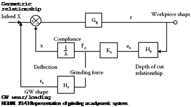
19.12.2 A Model of the Dynamic System
The dynamic system is represented in Figure 19.42 [Rowe 1979].
In Section 19.11.3, the geometry relationships were defined in terms of angle. A dynamic system also depends on time and acceleration. Referring to Section 19.11.5, the main relationships in terms of angular position on the workpiece are
Ideally, control wheel wear and workrest wear should be included in addition to the grinding wheel wear effect. However, these effects are usually much less significant.
Analysis of system stability starts from a general solution of waviness as a function that develops exponentially with time and has complex solutions of the complementary function of the form r(t) = c. ept. The roots of the complementary function have the form p = a+ jo. The real part, a, governs the growth rate of the system. A negative value implies a stable decay of the function. A positive value represents an unstable exponentially increasing value. The imaginary part, o, represents frequency. A zero value, a= 0, corresponds to solutions of the form r (t) = c ■ sin ot. This is a waviness condition of marginal stability and constant amplitude.
 |
If the system has an input function of the form u. = C ■ sin cot, the output of a linear stable system will have the form u0 = D ■ sin(ot + ф) where the amplitude is changed and there is a phase difference between the input and the output sine waves. It is important to realize that a sinusoidal forcing function at a frequency of marginal stability leads to an infinite response. A zero growth rate is, therefore, unstable.
Waviness expressed in terms of angle is r (в) = c ■ sin(2no/Q) = c ■ sin 2nn where Q is the workpiece speed in radians per second and n is the number of waves on the workpiece.
Transfer functions give the amplification and phase between the input and output for each block in the system. Gg gives the amplitude and phase of the wave produced at the grinding point for a sine wave input at the grinding point. Thus, if the feedback produces a workpiece reduction in radius in phase with the existing waviness, the amplitude will tend to grow. If the feedback produces a small reduction in radius in antiphase, the amplitude will tend to decay. A reduction in radius leading or lagging the existing waviness will create a wave that is constantly shifting around the workpiece periphery.
The denominator of a transfer function equated to zero is the characteristic equation of the system or subsystem. The characteristic equation expresses the condition for infinite amplitude response to a sine wave input.
In Laplace form, the transfer functions shown in Figure 19.43 are
Work-regenerative stability depends on the main feedback loop in Figure 19.43. The open-loop transfer function for the work-regenerative effect is the product of four terms. The main open-loop
transfer function in this case relates the vibration deflections x(s) fed back at the grinding point to the prescribed infeed motion X(s).
x( s) 1
—— = K———— G (s) ■ H (s) Open-loop transfer function (19.68)
X(s) s A(s) g a
At the limit of stability, the open-loop transfer function is equal to -1. The open-loop transfer function for limiting stability arranged in terms of angles and number of waves n is
The system compliance can be approximated for very low frequencies by writing A(s) = Я0. This is useful when the waviness corresponds to a frequency well below the principal machine resonance.
A similar open-loop transfer function may be written for the reduction in grinding wheel radius in the wheel regenerative loop.
= Ks • Gg(s) ■ Ha(s) ■ Hs(s) (19.70)
X(s) s g a
Wheel-regenerative vibration builds up waviness on the grinding wheel with increasing duration of grinding. When roundness errors exceed an acceptable level, the grinding wheel must be dressed to restore accuracy.